Taller de manejo de Datos en Pandas
Contents
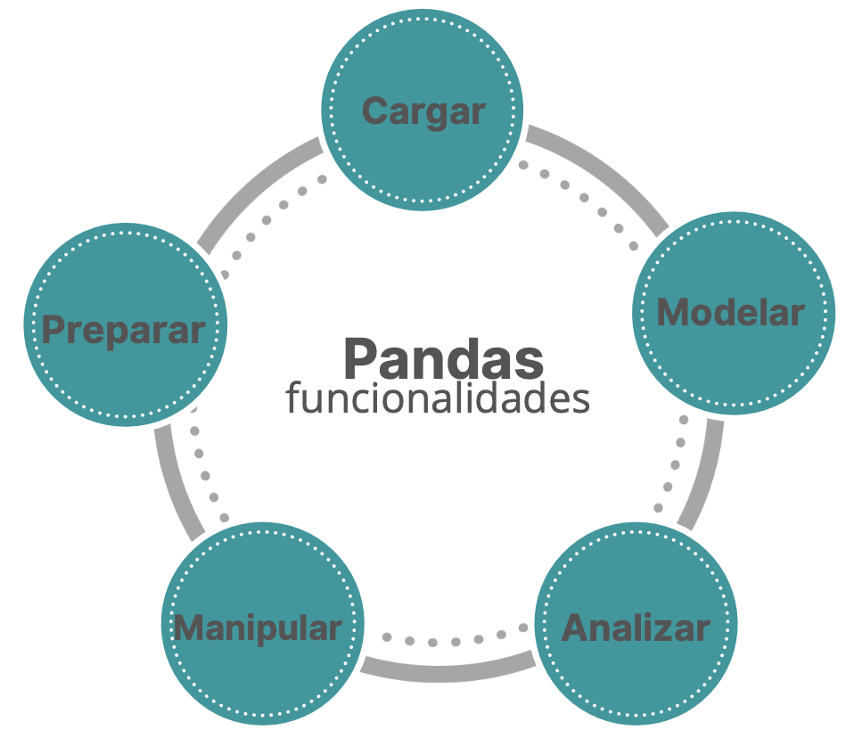
Taller de manejo de Datos en Pandas#
¿Qué es?#
Pandas es una librería de código abierto muy popular dentro del ámbito de Data Science y Machine Learning puesto que facilita el tratamiento y manipulación de datos.
Pandas nació de la necesidad de tener todas las funcionalidades necesarias para un analista de datos en una sola librería:
import pandas as pd
¿Cómo importar datos?#
Para leer los datos la estructura básica es pd.read_tipo-archivo. Si estamos en colab y queremos utilizar algunos datos que están en nuestro google drive podemos utilizar:
      from google.colab import drive
      drive.mount('/content/gdrive')
#from google.colab import ##drive correr solo en colab
#drive.mount('/content/gdrive')
counties = pd.read_excel("https://github.com/AprendizajeProfundo/Libro_Fundamentos_Programacion/blob/main/Python/Datos/counties.xlsx?raw=true")#cambiar dirección
Para tener una idea de qué variables y datos tengo en lo base de datos, sólo debemos llamarla.
counties
| codestate | codecounty | county | population | area | |
|---|---|---|---|---|---|
| 0 | 1 | 1001 | Auta#%&()uga | 54571.0 | 594.436000 |
| 1 | 1 | 1003 | Baldwin#%&() ? | 182265.0 | 1589.784000 |
| 2 | 1 | 1005 | Barbour | 27457.0 | 884.876000 |
| 3 | 1 | 1007 | Bi#%&()bb | 22915.0 | 622.582000 |
| 4 | 1 | 1009 | Blount ? | 57322.0 | 644.776000 |
| ... | ... | ... | ... | ... | ... |
| 3229 | 72 | 72151 | Yabucoa | 37941.0 | 55.215000 |
| 3230 | 72 | 72153 | Ya_uco | 42043.0 | 68.192000 |
| 3231 | 78 | 78010 | ; St. Croix ? | 50601.0 | 83.345868 |
| 3232 | 78 | 78020 | St. John | 4170.0 | 19.689867 |
| 3233 | 78 | 78030 | St. Thomas | 51634.0 | 31.313503 |
3234 rows × 5 columns
En lo anterior veiamos todas las variables con las 5 primeras y 5 últimas filas. Pero, podemos ver una cantidad determinada de registros tanto del inicio de la tabla como del final. Utlizando .head() y .tail() respectivamente.
counties.head(3) #por defecto salen 5 primeros
| codestate | codecounty | county | population | area | |
|---|---|---|---|---|---|
| 0 | 1 | 1001 | Auta#%&()uga | 54571.0 | 594.436 |
| 1 | 1 | 1003 | Baldwin#%&() ? | 182265.0 | 1589.784 |
| 2 | 1 | 1005 | Barbour | 27457.0 | 884.876 |
counties.tail(2)
| codestate | codecounty | county | population | area | |
|---|---|---|---|---|---|
| 3232 | 78 | 78020 | St. John | 4170.0 | 19.689867 |
| 3233 | 78 | 78030 | St. Thomas | 51634.0 | 31.313503 |
Si aparte de ver solamente la tabla, queremos más información de la base de datos, por ejemplo sus dimensiones y tipo de variables podemos utilizar lo siguiente:
counties.info()
print("\n")
print("La forma de la base de datos es:",counties.shape)  #shape:forma de un array
<class 'pandas.core.frame.DataFrame'>
RangeIndex: 3234 entries, 0 to 3233
Data columns (total 5 columns):
 #   Column      Non-Null Count  Dtype
---  ------      --------------  -----
 0   codestate   3234 non-null   int64
 1   codecounty  3234 non-null   int64
 2   county      3234 non-null   object
 3   population  3232 non-null   float64
 4   area        3234 non-null   float64
dtypes: float64(2), int64(2), object(1)
memory usage: 126.5+ KB


La forma de la base de datos es: (3234, 5)
print(counties.dtypes) #tipo de objeto en cada columna
print("\n")
print(counties.describe())
print("\n")
print(counties.describe(include="all")) #summary, si no se pone el include solo aparece de las variables numéricas
codestate       int64
codecounty      int64
county         object
population    float64
area          float64
dtype: object


         codestate    codecounty    population           area
count  3234.000000   3234.000000  3.232000e+03    3234.000000
mean     31.441868  31544.737786  9.679656e+04    1093.361817
std      16.411236  16425.545223  3.088044e+05    3564.706999
min       1.000000   1001.000000  1.700000e+01       0.031696
25%      19.000000  19039.500000  1.129700e+04     416.360000
50%      30.000000  30038.000000  2.607550e+04     602.977500
75%      46.000000  46128.500000  6.566050e+04     913.884500
max      78.000000  78030.000000  9.818605e+06  145504.789000


          codestate    codecounty    county    population           area
count   3234.000000   3234.000000      3234  3.232000e+03    3234.000000
unique          NaN           NaN      2625           NaN            NaN
top             NaN           NaN  Lincoln            NaN            NaN
freq            NaN           NaN        14           NaN            NaN
mean      31.441868  31544.737786       NaN  9.679656e+04    1093.361817
std       16.411236  16425.545223       NaN  3.088044e+05    3564.706999
min        1.000000   1001.000000       NaN  1.700000e+01       0.031696
25%       19.000000  19039.500000       NaN  1.129700e+04     416.360000
50%       30.000000  30038.000000       NaN  2.607550e+04     602.977500
75%       46.000000  46128.500000       NaN  6.566050e+04     913.884500
max       78.000000  78030.000000       NaN  9.818605e+06  145504.789000
Seleccionar subconjuntos de una base de datos#
Escoger columnas#
Para ver el nombre de las columnas que existen, podemos utilizar .columns.
counties.columns
Index(['codestate', 'codecounty', 'county', 'population', 'area'], dtype='object')
Escoger una columna específica o un conjunto de ellas
condado = counties["county"]
condado
0               Auta#%&()uga
1        Baldwin#%&()  ?
2                    Barbour
3                  Bi#%&()bb
4              Blount  ?
                ...
3229                 Yabucoa
3230                  Ya_uco
3231       ; St. Croix ?
3232                 St. John
3233               St. Thomas
Name: county, Length: 3234, dtype: object
print(condado.shape) #array unidimensional con 3234 elementos
print(counties["county"].shape)
print(type(condado))
(3234,)
(3234,)
<class 'pandas.core.series.Series'>
codi_condado=counties[["codecounty","county"]]
print(codi_condado)
print(type(codi_condado))
      codecounty                 county
0           1001          Auta#%&()uga
1           1003   Baldwin#%&()  ?
2           1005               Barbour
3           1007             Bi#%&()bb
4           1009         Blount  ?
...          ...                    ...
3229       72151               Yabucoa
3230       72153                Ya_uco
3231       78010     ; St. Croix ?
3232       78020               St. John
3233       78030             St. Thomas

[3234 rows x 2 columns]
<class 'pandas.core.frame.DataFrame'>
Escoger Filas#
Podemos escoger ciertas filas a través de su posición. utilizando .iloc
from seaborn import load_dataset
print(counties.iloc[0:1,])
print(type(counties.iloc[0:1,]))
   codestate  codecounty         county  population     area
0          1        1001  Auta#%&()uga      54571.0  594.436
<class 'pandas.core.frame.DataFrame'>
print(counties.iloc[8:12,1:3])
    codecounty                 county
8         1017     ; Chambers  ?
9         1019              Cherokee
10        1021             ; Chilton
11        1023               Choctaw
O también escoger filas con base a alguna condicion o característica específica.
counties.tail()
| codestate | codecounty | county | population | area | |
|---|---|---|---|---|---|
| 3229 | 72 | 72151 | Yabucoa | 37941.0 | 55.215000 |
| 3230 | 72 | 72153 | Ya_uco | 42043.0 | 68.192000 |
| 3231 | 78 | 78010 | ; St. Croix ? | 50601.0 | 83.345868 |
| 3232 | 78 | 78020 | St. John | 4170.0 | 19.689867 |
| 3233 | 78 | 78030 | St. Thomas | 51634.0 | 31.313503 |
counties["codestate"] > 72 #Verdadero o falso si cumple la condición
0       False
1       False
2       False
3       False
4       False
        ...
3229    False
3230    False
3231     True
3232     True
3233     True
Name: codestate, Length: 3234, dtype: bool
codsat72 = counties[counties["codestate"] > 72] # Llama aquellos cuyo valor es verdadero
codsat72.info()
<class 'pandas.core.frame.DataFrame'>
Int64Index: 3 entries, 3231 to 3233
Data columns (total 5 columns):
 #   Column      Non-Null Count  Dtype
---  ------      --------------  -----
 0   codestate   3 non-null      int64
 1   codecounty  3 non-null      int64
 2   county      3 non-null      object
 3   population  3 non-null      float64
 4   area        3 non-null      float64
dtypes: float64(2), int64(2), object(1)
memory usage: 144.0+ bytes
Filas que no tengan valores faltantes en determinada columna
no_na = counties[counties["population"].notna()]

print(no_na.shape)
print(counties.shape)
(3232, 5)
(3234, 5)
Filas con valores específicos#
Existen varias maneras de realizar estas búsquedas, algunas de ellas son utilizando isin, loc de la librería seaborn y or.
codcou1 = counties[counties["codecounty"].isin([78010, 72151])]
codcou1
| codestate | codecounty | county | population | area | |
|---|---|---|---|---|---|
| 3229 | 72 | 72151 | Yabucoa | 37941.0 | 55.215000 |
| 3231 | 78 | 78010 | ; St. Croix ? | 50601.0 | 83.345868 |
codcou2 = counties.loc[:, 'codecounty'] == 78010
codcou2_ = counties.loc[codcou2]
codcou2_
| codestate | codecounty | county | population | area | |
|---|---|---|---|---|---|
| 3231 | 78 | 78010 | ; St. Croix ? | 50601.0 | 83.345868 |
counties[(counties["codecounty"] == 78010) | (counties["codecounty"] == 72151)]
| codestate | codecounty | county | population | area | |
|---|---|---|---|---|---|
| 3229 | 72 | 72151 | Yabucoa | 37941.0 | 55.215000 |
| 3231 | 78 | 78010 | ; St. Croix ? | 50601.0 | 83.345868 |
Filas con más de una característica específica.
counties[(counties["codestate"] == 72) & (counties["area"] >= 60)].info()
<class 'pandas.core.frame.DataFrame'>
Int64Index: 16 entries, 3153 to 3230
Data columns (total 5 columns):
 #   Column      Non-Null Count  Dtype
---  ------      --------------  -----
 0   codestate   16 non-null     int64
 1   codecounty  16 non-null     int64
 2   county      16 non-null     object
 3   population  16 non-null     float64
 4   area        16 non-null     float64
dtypes: float64(2), int64(2), object(1)
memory usage: 768.0+ bytes
Eliminar valores omitidos#
#Eliminar valores omitidos: dropna
# axis= 0 -> Eliminar fila completa
# axis=1 -> Eliminar columna completa
counties.dropna(subset=["population"], axis=0, inplace=False) #inplace:modifique directamente la BD
| codestate | codecounty | county | population | area | |
|---|---|---|---|---|---|
| 0 | 1 | 1001 | Auta#%&()uga | 54571.0 | 594.436000 |
| 1 | 1 | 1003 | Baldwin#%&() ? | 182265.0 | 1589.784000 |
| 2 | 1 | 1005 | Barbour | 27457.0 | 884.876000 |
| 3 | 1 | 1007 | Bi#%&()bb | 22915.0 | 622.582000 |
| 4 | 1 | 1009 | Blount ? | 57322.0 | 644.776000 |
| ... | ... | ... | ... | ... | ... |
| 3229 | 72 | 72151 | Yabucoa | 37941.0 | 55.215000 |
| 3230 | 72 | 72153 | Ya_uco | 42043.0 | 68.192000 |
| 3231 | 78 | 78010 | ; St. Croix ? | 50601.0 | 83.345868 |
| 3232 | 78 | 78020 | St. John | 4170.0 | 19.689867 |
| 3233 | 78 | 78030 | St. Thomas | 51634.0 | 31.313503 |
3232 rows × 5 columns
Manipulación de datos textuales (Limpieza)#
Para realizarle limpieza a columna county de la base de datos counties, podemos utilizar lo siguiente:
**lower:**Poner en minúscula todo el texto.
**replace:**Remplazar ciertos valores por otros.
**strip:**Eliminar los espacios al principio y al final de la cadena.
**title:**Poner primera letra de cada palabra en mayúscula.
counties["county"] = (counties["county"]
                            .str.lower()
                            .str.replace("[^a-záéíóúüñ ]","")
                            .str.replace(" +"," ")
                            .str.strip()
                            .str.title()
                           )
/opt/hostedtoolcache/Python/3.7.13/x64/lib/python3.7/site-packages/ipykernel_launcher.py:3: FutureWarning: The default value of regex will change from True to False in a future version.
  This is separate from the ipykernel package so we can avoid doing imports until
/opt/hostedtoolcache/Python/3.7.13/x64/lib/python3.7/site-packages/ipykernel_launcher.py:4: FutureWarning: The default value of regex will change from True to False in a future version.
  after removing the cwd from sys.path.
print(counties)
      codestate  codecounty     county  population         area
0             1        1001    Autauga     54571.0   594.436000
1             1        1003    Baldwin    182265.0  1589.784000
2             1        1005    Barbour     27457.0   884.876000
3             1        1007       Bibb     22915.0   622.582000
4             1        1009     Blount     57322.0   644.776000
...         ...         ...        ...         ...          ...
3229         72       72151    Yabucoa     37941.0    55.215000
3230         72       72153      Yauco     42043.0    68.192000
3231         78       78010   St Croix     50601.0    83.345868
3232         78       78020    St John      4170.0    19.689867
3233         78       78030  St Thomas     51634.0    31.313503

[3234 rows x 5 columns]
Creación de columnas a partir de otras#
counties["densidad"]= counties["population"]/counties["area"]
print(counties[["densidad","population","area"]])
         densidad  population         area
0       91.802986     54571.0   594.436000
1      114.647650    182265.0  1589.784000
2       31.029206     27457.0   884.876000
3       36.806397     22915.0   622.582000
4       88.902192     57322.0   644.776000
...           ...         ...          ...
3229   687.150231     37941.0    55.215000
3230   616.538597     42043.0    68.192000
3231   607.120676     50601.0    83.345868
3232   211.784062      4170.0    19.689867
3233  1648.937201     51634.0    31.313503

[3234 rows x 3 columns]
Renombrar columnas#
print(counties.columns)
counties.rename(columns={"densidad":"densidad_pob"},inplace=True) #renombrar columna
print(counties.columns) #Verificación
Index(['codestate', 'codecounty', 'county', 'population', 'area', 'densidad'], dtype='object')
Index(['codestate', 'codecounty', 'county', 'population', 'area',
       'densidad_pob'],
      dtype='object')
Modificar tipo de dato de una columna#
print(counties.info())
print("\n")
counties["codestate"]=counties["codestate"].astype("float")
print(counties.info())
<class 'pandas.core.frame.DataFrame'>
RangeIndex: 3234 entries, 0 to 3233
Data columns (total 6 columns):
 #   Column        Non-Null Count  Dtype
---  ------        --------------  -----
 0   codestate     3234 non-null   int64
 1   codecounty    3234 non-null   int64
 2   county        3234 non-null   object
 3   population    3232 non-null   float64
 4   area          3234 non-null   float64
 5   densidad_pob  3232 non-null   float64
dtypes: float64(3), int64(2), object(1)
memory usage: 151.7+ KB
None


<class 'pandas.core.frame.DataFrame'>
RangeIndex: 3234 entries, 0 to 3233
Data columns (total 6 columns):
 #   Column        Non-Null Count  Dtype
---  ------        --------------  -----
 0   codestate     3234 non-null   float64
 1   codecounty    3234 non-null   int64
 2   county        3234 non-null   object
 3   population    3232 non-null   float64
 4   area          3234 non-null   float64
 5   densidad_pob  3232 non-null   float64
dtypes: float64(4), int64(1), object(1)
memory usage: 151.7+ KB
None
Eliminar filas y columnas#
Eliminación filas, puede ser por posición o que cumpla una característica.
print(counties.shape)
counties = counties.drop(counties.iloc[0:3,].index)
counties = counties.drop(counties[counties['codecounty']==70].index)
print(counties.shape)
(3234, 6)
(3231, 6)
counties.drop(['densidad_pob'], axis=1,inplace=True) #inplace=True, para que me modifique la BD
counties.columns
Index(['codestate', 'codecounty', 'county', 'population', 'area'], dtype='object')
Conteos#
La función groupby devuelve un objeto DataFrameGroupBy que contiene la información agrupada según las especificaciones que indiquemos.
group=counties.groupby("codestate")
print(type(group))
<class 'pandas.core.groupby.generic.DataFrameGroupBy'>
Podemos obtener detalles del anterior dataframe
print(group.first().head(10)) # Nos muestra el primer elemento de cada grupo según "codestate"
print('\n')
print(group.get_group(78)) #Nos muestra los elementos cuyo codestate es 78
           codecounty                county  population       area
codestate
1.0              1007                  Bibb     22915.0    622.582
2.0              2013        Aleutians East      3141.0   6981.943
4.0              4001                Apache     71518.0  11197.521
5.0              5001              Arkansas     19019.0    988.770
6.0              6001               Alameda   1510271.0    739.017
8.0              8001                 Adams    441603.0   1167.653
9.0              9001             Fairfield    916829.0    624.890
10.0            10001                  Kent    162310.0    586.179
11.0            11001  District Of Columbia    601723.0     61.048
12.0            12001               Alachua    247336.0    875.020


      codestate  codecounty     county  population       area
3231       78.0       78010   St Croix     50601.0  83.345868
3232       78.0       78020    St John      4170.0  19.689867
3233       78.0       78030  St Thomas     51634.0  31.313503
counties.groupby("codestate")["codecounty"].count().head(10)
codestate
1.0     64
2.0     29
4.0     15
5.0     75
6.0     58
8.0     64
9.0      8
10.0     3
11.0     1
12.0    67
Name: codecounty, dtype: int64
Modificar Tablas#
es posible hacer cambios de orden y estructura en las tablas de pandas.
folder_path="https://github.com/AprendizajeProfundo/Libro_Fundamentos_Programacion/blob/main/Python/Datos/"
elections=pd.read_excel(folder_path+'elections.xlsx?raw=true')
elections.head(5)
| year | democrat | republic | other | codecounty | |
|---|---|---|---|---|---|
| 0 | 2000 | 4942 | 11993 | 273 | 1001 |
| 1 | 2000 | 13997 | 40872 | 1611 | 1003 |
| 2 | 2000 | 5188 | 5096 | 111 | 1005 |
| 3 | 2000 | 2710 | 4273 | 118 | 1007 |
| 4 | 2000 | 4977 | 12667 | 329 | 1009 |
organicemos los datos descendentemente depende de la cantidad de votos democratas
elections.sort_values(["democrat"], ascending=False)
| year | democrat | republic | other | codecounty | |
|---|---|---|---|---|---|
| 12626 | 2016 | 2464364 | 769743 | 200201 | 6037 |
| 6400 | 2008 | 2295853 | 956425 | 65970 | 6037 |
| 9513 | 2012 | 2216903 | 885333 | 78831 | 6037 |
| 3287 | 2004 | 1907736 | 1076225 | 37686 | 6037 |
| 175 | 2000 | 1710505 | 871930 | 112719 | 6037 |
| ... | ... | ... | ... | ... | ... |
| 11981 | 2012 | 9 | 54 | 1 | 48301 |
| 8852 | 2008 | 8 | 151 | 4 | 48269 |
| 11965 | 2012 | 5 | 139 | 1 | 48269 |
| 15078 | 2016 | 5 | 149 | 5 | 48269 |
| 15094 | 2016 | 4 | 58 | 3 | 48301 |
15563 rows × 5 columns
usando groupby() podemos juntar los datos por año y sumarlos para tener el total de votos por año
elections.groupby('year')[['democrat', 'republic']].sum()
| democrat | republic | |
|---|---|---|
| year | ||
| 2000 | 50922964 | 50290498 |
| 2004 | 58614073 | 61603653 |
| 2008 | 69204582 | 59703000 |
| 2012 | 65508961 | 60460609 |
| 2016 | 65626398 | 62790289 |
Podemos aplicar ambos métodos en un mismo código
elections_sort=(elections.groupby('year')[['democrat', 'republic']]
                .sum()
                .sort_values('democrat', ascending=False))
display(elections_sort)
| democrat | republic | |
|---|---|---|
| year | ||
| 2008 | 69204582 | 59703000 |
| 2016 | 65626398 | 62790289 |
| 2012 | 65508961 | 60460609 |
| 2004 | 58614073 | 61603653 |
| 2000 | 50922964 | 50290498 |
Para reestructurar los datos usamos la función pivot().
pivot_elections=elections.pivot(index='codecounty',
                columns='year',
                values=['democrat','republic'])
pivot_elections.head()
| democrat | republic | |||||||||
|---|---|---|---|---|---|---|---|---|---|---|
| year | 2000 | 2004 | 2008 | 2012 | 2016 | 2000 | 2004 | 2008 | 2012 | 2016 |
| codecounty | ||||||||||
| 1001 | 4942.0 | 4758.0 | 6093.0 | 6363.0 | 5936.0 | 11993.0 | 15196.0 | 17403.0 | 17379.0 | 18172.0 |
| 1003 | 13997.0 | 15599.0 | 19386.0 | 18424.0 | 18458.0 | 40872.0 | 52971.0 | 61271.0 | 66016.0 | 72883.0 |
| 1005 | 5188.0 | 4832.0 | 5697.0 | 5912.0 | 4871.0 | 5096.0 | 5899.0 | 5866.0 | 5550.0 | 5454.0 |
| 1007 | 2710.0 | 2089.0 | 2299.0 | 2202.0 | 1874.0 | 4273.0 | 5472.0 | 6262.0 | 6132.0 | 6738.0 |
| 1009 | 4977.0 | 3938.0 | 3522.0 | 2970.0 | 2156.0 | 12667.0 | 17386.0 | 20389.0 | 20757.0 | 22859.0 |
Múltiples índices#
Se pueden elegir múltiples variables como índice del dataframe. Esto es util para facilitar la extracción de información en ciertos casos
counties_multi=pd.read_excel(folder_path+"counties.xlsx?raw=true", index_col=[0, 1])
display(counties_multi)
| county | population | area | ||
|---|---|---|---|---|
| codestate | codecounty | |||
| 1 | 1001 | Auta#%&()uga | 54571.0 | 594.436000 |
| 1003 | Baldwin#%&() ? | 182265.0 | 1589.784000 | |
| 1005 | Barbour | 27457.0 | 884.876000 | |
| 1007 | Bi#%&()bb | 22915.0 | 622.582000 | |
| 1009 | Blount ? | 57322.0 | 644.776000 | |
| ... | ... | ... | ... | ... |
| 72 | 72151 | Yabucoa | 37941.0 | 55.215000 |
| 72153 | Ya_uco | 42043.0 | 68.192000 | |
| 78 | 78010 | ; St. Croix ? | 50601.0 | 83.345868 |
| 78020 | St. John | 4170.0 | 19.689867 | |
| 78030 | St. Thomas | 51634.0 | 31.313503 |
3234 rows × 3 columns
Podemos obtener la suma de población de cada estado
counties_multi['population'].sum(level='codestate').head(5)
/opt/hostedtoolcache/Python/3.7.13/x64/lib/python3.7/site-packages/ipykernel_launcher.py:1: FutureWarning: Using the level keyword in DataFrame and Series aggregations is deprecated and will be removed in a future version. Use groupby instead. df.sum(level=1) should use df.groupby(level=1).sum().
  """Entry point for launching an IPython kernel.
codestate
1     4779736.0
2      710231.0
4     6392017.0
5     2915918.0
6    37253956.0
Name: population, dtype: float64
Concatenar y unir#
Es posible unir varias tablas tanto vertical como horizontalmente.
En ambos casos, podemos usar concat(), y se juntarán las bases con bases a los nombres de columnas o los indices de las filas
elections_2000=elections[elections['year']==2000]
display(elections_2000) #display:ejecuta el método dunder apropiado para obtener los datos apropiados para mostrar
| year | democrat | republic | other | codecounty | |
|---|---|---|---|---|---|
| 0 | 2000 | 4942 | 11993 | 273 | 1001 |
| 1 | 2000 | 13997 | 40872 | 1611 | 1003 |
| 2 | 2000 | 5188 | 5096 | 111 | 1005 |
| 3 | 2000 | 2710 | 4273 | 118 | 1007 |
| 4 | 2000 | 4977 | 12667 | 329 | 1009 |
| ... | ... | ... | ... | ... | ... |
| 3107 | 2000 | 5521 | 9425 | 745 | 56037 |
| 3108 | 2000 | 4019 | 5454 | 958 | 56039 |
| 3109 | 2000 | 1650 | 5469 | 299 | 56041 |
| 3110 | 2000 | 806 | 3138 | 107 | 56043 |
| 3111 | 2000 | 449 | 2521 | 90 | 56045 |
3112 rows × 5 columns
elections_2004=elections[elections['year']==2004]
elections_2004['dummy']=0
display(elections_2004)
/opt/hostedtoolcache/Python/3.7.13/x64/lib/python3.7/site-packages/ipykernel_launcher.py:2: SettingWithCopyWarning:
A value is trying to be set on a copy of a slice from a DataFrame.
Try using .loc[row_indexer,col_indexer] = value instead

See the caveats in the documentation: https://pandas.pydata.org/pandas-docs/stable/user_guide/indexing.html#returning-a-view-versus-a-copy
| year | democrat | republic | other | codecounty | dummy | |
|---|---|---|---|---|---|---|
| 3112 | 2004 | 4758 | 15196 | 127 | 1001 | 0 |
| 3113 | 2004 | 15599 | 52971 | 750 | 1003 | 0 |
| 3114 | 2004 | 4832 | 5899 | 46 | 1005 | 0 |
| 3115 | 2004 | 2089 | 5472 | 39 | 1007 | 0 |
| 3116 | 2004 | 3938 | 17386 | 180 | 1009 | 0 |
| ... | ... | ... | ... | ... | ... | ... |
| 6220 | 2004 | 5208 | 10653 | 411 | 56037 | 0 |
| 6221 | 2004 | 5972 | 5124 | 263 | 56039 | 0 |
| 6222 | 2004 | 1815 | 6081 | 185 | 56041 | 0 |
| 6223 | 2004 | 855 | 3200 | 59 | 56043 | 0 |
| 6224 | 2004 | 580 | 2739 | 73 | 56045 | 0 |
3113 rows × 6 columns
Si se hace la concatenación sin más, se tomarán todas las columnas y se agregarán NaN
elections_00_04=pd.concat([elections_2000, elections_2004])
display(elections_00_04)
| year | democrat | republic | other | codecounty | dummy | |
|---|---|---|---|---|---|---|
| 0 | 2000 | 4942 | 11993 | 273 | 1001 | NaN |
| 1 | 2000 | 13997 | 40872 | 1611 | 1003 | NaN |
| 2 | 2000 | 5188 | 5096 | 111 | 1005 | NaN |
| 3 | 2000 | 2710 | 4273 | 118 | 1007 | NaN |
| 4 | 2000 | 4977 | 12667 | 329 | 1009 | NaN |
| ... | ... | ... | ... | ... | ... | ... |
| 6220 | 2004 | 5208 | 10653 | 411 | 56037 | 0.0 |
| 6221 | 2004 | 5972 | 5124 | 263 | 56039 | 0.0 |
| 6222 | 2004 | 1815 | 6081 | 185 | 56041 | 0.0 |
| 6223 | 2004 | 855 | 3200 | 59 | 56043 | 0.0 |
| 6224 | 2004 | 580 | 2739 | 73 | 56045 | 0.0 |
6225 rows × 6 columns
Ahora, usando merge(), podemos hacer uniones de las tablas de forma horizontal que compartan una columna/indice en común
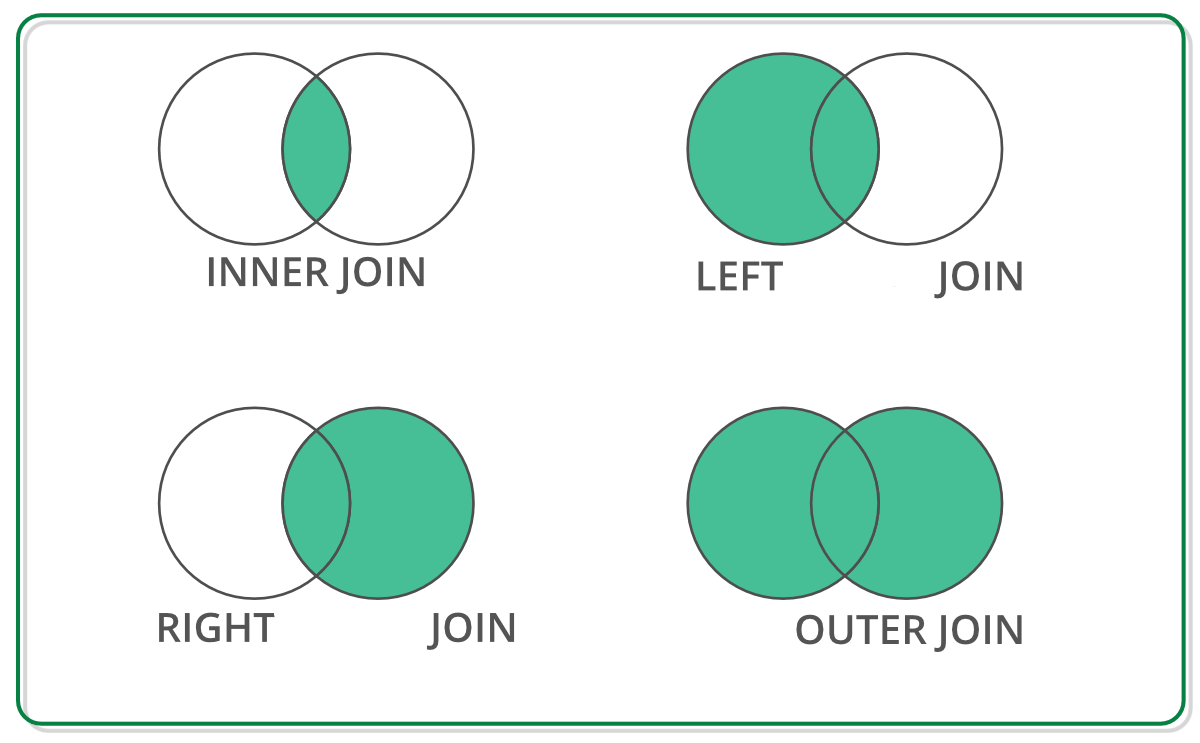
Tipos de Joins
display(counties)
| codestate | codecounty | county | population | area | |
|---|---|---|---|---|---|
| 3 | 1.0 | 1007 | Bibb | 22915.0 | 622.582000 |
| 4 | 1.0 | 1009 | Blount | 57322.0 | 644.776000 |
| 5 | 1.0 | 1011 | Bullock | 10914.0 | 622.805000 |
| 6 | 1.0 | 1013 | Butler | 20947.0 | 776.829000 |
| 7 | 1.0 | 1015 | Calhoun | 118572.0 | 605.868000 |
| ... | ... | ... | ... | ... | ... |
| 3229 | 72.0 | 72151 | Yabucoa | 37941.0 | 55.215000 |
| 3230 | 72.0 | 72153 | Yauco | 42043.0 | 68.192000 |
| 3231 | 78.0 | 78010 | St Croix | 50601.0 | 83.345868 |
| 3232 | 78.0 | 78020 | St John | 4170.0 | 19.689867 |
| 3233 | 78.0 | 78030 | St Thomas | 51634.0 | 31.313503 |
3231 rows × 5 columns
inner_joined=pd.merge(elections, counties)
inner_joined.head(10)
| year | democrat | republic | other | codecounty | codestate | county | population | area | |
|---|---|---|---|---|---|---|---|---|---|
| 0 | 2000 | 2710 | 4273 | 118 | 1007 | 1.0 | Bibb | 22915.0 | 622.582 |
| 1 | 2004 | 2089 | 5472 | 39 | 1007 | 1.0 | Bibb | 22915.0 | 622.582 |
| 2 | 2008 | 2299 | 6262 | 83 | 1007 | 1.0 | Bibb | 22915.0 | 622.582 |
| 3 | 2012 | 2202 | 6132 | 86 | 1007 | 1.0 | Bibb | 22915.0 | 622.582 |
| 4 | 2016 | 1874 | 6738 | 207 | 1007 | 1.0 | Bibb | 22915.0 | 622.582 |
| 5 | 2000 | 4977 | 12667 | 329 | 1009 | 1.0 | Blount | 57322.0 | 644.776 |
| 6 | 2004 | 3938 | 17386 | 180 | 1009 | 1.0 | Blount | 57322.0 | 644.776 |
| 7 | 2008 | 3522 | 20389 | 356 | 1009 | 1.0 | Blount | 57322.0 | 644.776 |
| 8 | 2012 | 2970 | 20757 | 279 | 1009 | 1.0 | Blount | 57322.0 | 644.776 |
| 9 | 2016 | 2156 | 22859 | 573 | 1009 | 1.0 | Blount | 57322.0 | 644.776 |
outer_joined=pd.merge(elections, counties, how='outer')
outer_joined.head(10)
| year | democrat | republic | other | codecounty | codestate | county | population | area | |
|---|---|---|---|---|---|---|---|---|---|
| 0 | 2000.0 | 4942.0 | 11993.0 | 273.0 | 1001 | NaN | NaN | NaN | NaN |
| 1 | 2004.0 | 4758.0 | 15196.0 | 127.0 | 1001 | NaN | NaN | NaN | NaN |
| 2 | 2008.0 | 6093.0 | 17403.0 | 145.0 | 1001 | NaN | NaN | NaN | NaN |
| 3 | 2012.0 | 6363.0 | 17379.0 | 190.0 | 1001 | NaN | NaN | NaN | NaN |
| 4 | 2016.0 | 5936.0 | 18172.0 | 865.0 | 1001 | NaN | NaN | NaN | NaN |
| 5 | 2000.0 | 13997.0 | 40872.0 | 1611.0 | 1003 | NaN | NaN | NaN | NaN |
| 6 | 2004.0 | 15599.0 | 52971.0 | 750.0 | 1003 | NaN | NaN | NaN | NaN |
| 7 | 2008.0 | 19386.0 | 61271.0 | 756.0 | 1003 | NaN | NaN | NaN | NaN |
| 8 | 2012.0 | 18424.0 | 66016.0 | 898.0 | 1003 | NaN | NaN | NaN | NaN |
| 9 | 2016.0 | 18458.0 | 72883.0 | 3874.0 | 1003 | NaN | NaN | NaN | NaN |
left_joined=pd.merge(elections, counties, how='left')
left_joined.head(10)
| year | democrat | republic | other | codecounty | codestate | county | population | area | |
|---|---|---|---|---|---|---|---|---|---|
| 0 | 2000 | 4942 | 11993 | 273 | 1001 | NaN | NaN | NaN | NaN |
| 1 | 2000 | 13997 | 40872 | 1611 | 1003 | NaN | NaN | NaN | NaN |
| 2 | 2000 | 5188 | 5096 | 111 | 1005 | NaN | NaN | NaN | NaN |
| 3 | 2000 | 2710 | 4273 | 118 | 1007 | 1.0 | Bibb | 22915.0 | 622.582 |
| 4 | 2000 | 4977 | 12667 | 329 | 1009 | 1.0 | Blount | 57322.0 | 644.776 |
| 5 | 2000 | 3395 | 1433 | 76 | 1011 | 1.0 | Bullock | 10914.0 | 622.805 |
| 6 | 2000 | 3606 | 4127 | 70 | 1013 | 1.0 | Butler | 20947.0 | 776.829 |
| 7 | 2000 | 15781 | 22306 | 822 | 1015 | 1.0 | Calhoun | 118572.0 | 605.868 |
| 8 | 2000 | 5616 | 6037 | 181 | 1017 | 1.0 | Chambers | 34215.0 | 596.531 |
| 9 | 2000 | 3497 | 4154 | 172 | 1019 | 1.0 | Cherokee | 25989.0 | 553.700 |
right_joined=pd.merge(elections, counties, how='right')
right_joined.head(10)
| year | democrat | republic | other | codecounty | codestate | county | population | area | |
|---|---|---|---|---|---|---|---|---|---|
| 0 | 2000.0 | 2710.0 | 4273.0 | 118.0 | 1007 | 1.0 | Bibb | 22915.0 | 622.582 |
| 1 | 2004.0 | 2089.0 | 5472.0 | 39.0 | 1007 | 1.0 | Bibb | 22915.0 | 622.582 |
| 2 | 2008.0 | 2299.0 | 6262.0 | 83.0 | 1007 | 1.0 | Bibb | 22915.0 | 622.582 |
| 3 | 2012.0 | 2202.0 | 6132.0 | 86.0 | 1007 | 1.0 | Bibb | 22915.0 | 622.582 |
| 4 | 2016.0 | 1874.0 | 6738.0 | 207.0 | 1007 | 1.0 | Bibb | 22915.0 | 622.582 |
| 5 | 2000.0 | 4977.0 | 12667.0 | 329.0 | 1009 | 1.0 | Blount | 57322.0 | 644.776 |
| 6 | 2004.0 | 3938.0 | 17386.0 | 180.0 | 1009 | 1.0 | Blount | 57322.0 | 644.776 |
| 7 | 2008.0 | 3522.0 | 20389.0 | 356.0 | 1009 | 1.0 | Blount | 57322.0 | 644.776 |
| 8 | 2012.0 | 2970.0 | 20757.0 | 279.0 | 1009 | 1.0 | Blount | 57322.0 | 644.776 |
| 9 | 2016.0 | 2156.0 | 22859.0 | 573.0 | 1009 | 1.0 | Blount | 57322.0 | 644.776 |
Series de tiempo y time stamps#
Existe un tipo de datos llamado “timestamp” que se usa para medir registros de tiempo. Es posible pasar strings a este tipo de dato en diferentes formatos y trabajar con este usándolo como indice
airrpm=pd.read_csv(folder_path+'airrpm.txt?raw=true', header=None, delimiter= '\s+', decimal=",")
airrpm.columns=["Time", "R1", "R2", "R3"]
airrpm.head()
| Time | R1 | R2 | R3 | |
|---|---|---|---|---|
| 0 | Jan-79 | 26.64 | 15.50 | 11.15 |
| 1 | Feb-79 | 27.20 | 16.58 | 10.62 |
| 2 | Mar-79 | 27.87 | 18.85 | 9.02 |
| 3 | Apr-79 | 23.22 | 17.23 | 5.99 |
| 4 | May-79 | 23.27 | 16.04 | 7.23 |
La variable “Time” en este momento es un string. Pero podemos transformarlo usando to_datetime(). Para obtener más información de qué se podría poner en format, pueden revisar este link
airrpm['Time']=pd.to_datetime(airrpm['Time'], format='%b-%y')
airrpm.index=airrpm['Time']
airrpm=airrpm.drop(['Time'], axis=1)
airrpm.head()
| R1 | R2 | R3 | |
|---|---|---|---|
| Time | |||
| 1979-01-01 | 26.64 | 15.50 | 11.15 |
| 1979-02-01 | 27.20 | 16.58 | 10.62 |
| 1979-03-01 | 27.87 | 18.85 | 9.02 |
| 1979-04-01 | 23.22 | 17.23 | 5.99 |
| 1979-05-01 | 23.27 | 16.04 | 7.23 |
Definiendo la fecha como índice, podemos extraer información con respecto al año y respecto al mes
airrpm.groupby([airrpm.index.month])['R1'].describe()
| count | mean | std | min | 25% | 50% | 75% | max | |
|---|---|---|---|---|---|---|---|---|
| Time | ||||||||
| 1 | 26.0 | 43.736538 | 9.778402 | 26.64 | 36.6575 | 44.82 | 51.86 | 59.36 |
| 2 | 25.0 | 43.680800 | 9.983696 | 27.20 | 35.5400 | 44.74 | 52.73 | 59.74 |
| 3 | 25.0 | 44.514400 | 10.363336 | 27.87 | 35.7000 | 45.01 | 53.26 | 60.10 |
| 4 | 25.0 | 44.287200 | 10.480331 | 23.22 | 36.6100 | 45.63 | 52.79 | 60.49 |
| 5 | 25.0 | 43.891600 | 10.524814 | 23.27 | 34.6000 | 45.11 | 52.57 | 60.36 |
| 6 | 25.0 | 45.655600 | 10.586951 | 27.30 | 35.4200 | 47.29 | 54.55 | 61.88 |
| 7 | 25.0 | 46.478400 | 10.333910 | 29.28 | 38.2700 | 47.79 | 54.94 | 63.02 |
| 8 | 25.0 | 46.773600 | 10.613169 | 27.27 | 38.8600 | 48.06 | 55.39 | 63.71 |
| 9 | 25.0 | 44.202400 | 9.731246 | 27.13 | 37.2600 | 46.39 | 51.83 | 59.54 |
| 10 | 25.0 | 44.433200 | 10.093832 | 26.97 | 37.8500 | 45.89 | 51.56 | 60.26 |
| 11 | 25.0 | 43.841200 | 9.923719 | 26.19 | 37.3300 | 45.50 | 51.02 | 59.21 |
| 12 | 25.0 | 44.600400 | 9.573277 | 27.32 | 38.7500 | 45.33 | 51.98 | 57.65 |
airrpm.groupby([airrpm.index.year]).sum().head(10)
| R1 | R2 | R3 | |
|---|---|---|---|
| Time | |||
| 1979 | 328.83 | 210.49 | 118.34 |
| 1980 | 340.95 | 200.92 | 140.05 |
| 1981 | 341.96 | 198.53 | 143.45 |
| 1982 | 355.17 | 210.23 | 144.91 |
| 1983 | 374.03 | 226.76 | 147.26 |
| 1984 | 415.88 | 243.71 | 172.18 |
| 1985 | 440.43 | 271.80 | 168.61 |
| 1986 | 492.37 | 302.20 | 190.18 |
| 1987 | 522.07 | 324.58 | 197.52 |
| 1988 | 530.25 | 328.69 | 201.57 |